
eJournal of Tax Research

|
|
Home
| Databases
| WorldLII
| Search
| Feedback
eJournal of Tax Research |
|
The Marginal Cost of Public Funds for Excise Taxes in Thailand[†]
Worawan Chandoevwit[∗] and Bev Dahlby∗∗
Abstract
We extend the Ahmad and Stern (1984) framework for calculating the marginal cost of public funds (MCF) for excise taxes in Thailand by incorporating non-tax distortions caused by (a) environmental externalities, (b) public expenditure externalities, (c) market power in setting prices, (d) addiction, and (e) smuggling or tax evasion. Our calculations, based on our benchmark parameter values, indicates that the MCFs are 0.532 for fuel excise taxes, 2.187 for tobacco excise taxes, 2.132 for alcohol excise taxes and 1.080 for the VAT. Using pro-poor distributional weights does not change the relative social marginal cost of raising revenues through the excise taxes.
Excise taxes, commodity taxes, and import duties are the most important sources of tax revenue in most developing countries, represented 60.6 percent of tax revenues in developing countries in 1995-97 compared to 32.5 percent in OECD countries.[1] Among Southeast Asian countries, reliance on taxes on goods and services ranges from 13.0 percent of total tax revenue in Brunei to 82.3 percent in Cambodia. In Thailand, commodity taxes represent 59.1 percent of total tax revenues, with excise taxes contributing 25.6 percent of tax revenues. Given its heavy reliance on excise taxes, the equity and efficiency effects of excise taxes are important aspects of tax policy in Thailand. In this paper, we contribute to the analysis of excise tax policy in Thailand by computing the marginal cost of public funds (MCF) for the excise taxes on alcohol, tobacco, and fuel and for the value-added tax. We utilize the basic analytical framework for measuring the MCFs developed by Ahmad and Stern (1984) by using estimates of the own-and cross-price elasticities of demand for 10 categories of goods and services in Thailand. This allows us to capture the interdependence of the various commodity tax bases in Thailand in computing the MCFs. In addition, we extend the basic Ahmad and Stern framework by incorporating in the computation of the MCFs the non-tax distortions created by (a) environmental externalities, (b) public expenditure externalities, (c) addiction, (d) market power, and (e) smuggling. Our analysis, based on our benchmark parameter values, indicates that the MCFs are 0.532 for fuel excise taxes, 2.187 for tobacco excise taxes, 2.312 for alcohol excise taxes, and 1.080 for a VAT increase. We also use pro-poor distributional weights and data on the spending patterns of 90 household groups in Thailand to calculate distributionally-weighted MCFs, but this procedure does not change the ranking of the social marginal cost of the excise taxes. Finally, we show that a revenue-neutral marginal tax reform—reducing the excise tax rates on alcohol and tobacco by one percentage point and increasing the fuel excise tax—would result in a net efficiency gain equal to 1.72 Baht for every additional Baht of fuel tax revenue.
The paper is organized as follows. The next section outlines the basic theory of the MCF and how we incorporate the various non-tax distortions, such as externalities, market power, smuggling and addiction, in the formula for the MCF. Then we describe the parameters used in the calculations—tax rates, budget shares, elasticities of demand, and measures of the non-tax distortions. In the subsequent section, we present our calculations of the MCFs, including the contributions of the various non-tax distortions to the overall MCFs, and the potential net gain from a revenue neutral marginal tax reform. The penultimate section describes the computations of the distributionally-weighted MCFs. The final section contains our conclusions.
THE THEORY OF THE MCF[2]
The marginal cost of public funds measures the loss incurred by society in raising additional tax revenues. It has emerged as one of the most important concepts in the field of public economics, playing a key role in the evaluation of tax reforms, public expenditure programs, and other public policies, ranging from tax enforcement to privatization.
Tax Distortions
Taxes can distort the allocation of resources in an economy by altering taxpayers’ consumption, savings, labor supply, and investment decisions. The MCF is a summary measure of the additional distortion in the allocation of resources that occurs when a government raises additional revenue. However, minimizing the efficiency losses is not the only criteria for evaluating tax measures because taxes that impose heavy burdens on low income individuals are also “costly” taxes. The MCF concept can be used to combine equity or distributional concerns with efficiency effects in a summary measure of the total cost to a society of raising tax revenue. In this paper we use the MCF concept to evaluate the main excise taxes imposed by the government of Thailand.
Our basic model follows the approach pioneered by Ahmad and Stern (1984). For general surveys of the methodology and issues in evaluating commodity tax reforms, see Ray (1997), Santoro (no date) and Dahlby (forthcoming, Ch. 3). Our main methodological contribution is the inclusion of non-tax distortions in the computation of the MCFs for excise taxes. Initially, to simplify the analysis, we will ignore distributional issues by assuming that the economy only consists of one individual whose well-being is represented by the indirect utility function, V(q, I), where q is the vector of consumer prices and I is lump-sum income. Later we show how to incorporate distributional concerns in the measurement of the social marginal cost of public funds (SMCF).
Total tax revenues ![]() depend on the tax rates, ti, imposed on
the n commodities, denoted by the xis, that are consumed by the
individual. A money measure of the harm imposed on the individual in raising an
extra dollar of tax revenue
by increasing tax rate ti is defined by
the expression:
depend on the tax rates, ti, imposed on
the n commodities, denoted by the xis, that are consumed by the
individual. A money measure of the harm imposed on the individual in raising an
extra dollar of tax revenue
by increasing tax rate ti is defined by
the expression:
 (1)
(1)
where ![]() is the individual’s marginal utility of income. In defining
the
is the individual’s marginal utility of income. In defining
the![]() , it is assumed that dR/dti is positive, i.e. that the
government is operating on the upward-sloping section of its Laffer curve with
respect to ti.
, it is assumed that dR/dti is positive, i.e. that the
government is operating on the upward-sloping section of its Laffer curve with
respect to ti.
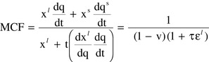
If a tax increase is fully reflected in the consumer price of the product and
does not affect the prices of other products―dqi/dti
= 1 and dqj/dti = 0―and using Roy’s theorem,
the following expression for the ![]() can be
derived:[3]
can be
derived:[3]
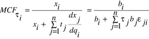 (2)
(2)
where εji is the elasticity of demand for commodity j with
respect to the price of commodity i, bj is the budget share of
commodity j, and τj = tj/qj is the ad
valorem tax rate on commodity j. This expression for the MCF indicates the
importance of the tax rates on other commodities
in evaluating the MCF for any
particular commodity tax. If commodity j is a substitute for commodity i and
![]() ,
then an increase in the tax on commodity i will boost the demand for commodity
j. The additional tax revenue collected from the
tax on commodity j is a
measure of the welfare gain from the improvement in the allocation of resources
in the jth commodity market
arising from the increase in ti, and this
effect reduces the MCFti. Conversely, if the commodity j is a
complement for i, then raising the tax rate on commodity i will exacerbate the
tax distortion
in the allocation of resources in the jth commodity market by
reducing the consumption of j. The resulting loss of revenue from
the tax on j
is a measure of the additional distortion caused by the tax increase on
commodity i.
,
then an increase in the tax on commodity i will boost the demand for commodity
j. The additional tax revenue collected from the
tax on commodity j is a
measure of the welfare gain from the improvement in the allocation of resources
in the jth commodity market
arising from the increase in ti, and this
effect reduces the MCFti. Conversely, if the commodity j is a
complement for i, then raising the tax rate on commodity i will exacerbate the
tax distortion
in the allocation of resources in the jth commodity market by
reducing the consumption of j. The resulting loss of revenue from
the tax on j
is a measure of the additional distortion caused by the tax increase on
commodity i.
The theory of optimal commodity taxation emphasizes the interaction between the demands for the taxed commodity and leisure. In particular, the Corlett and Hague Rule for optimal commodity taxation states that higher taxes should be levied on the commodities that are more complementary with leisure in order to offset the distortion in the labour-leisure decision caused by our inability to tax leisure directly. We will consider the implications of the interaction between commodity taxes and leisure-labour supply decisions for the measurement of the MCFs for excise taxes in the section dealing with the estimation of the demand elasticities.
As Devarajan et al (2001) have stressed, it is very important to consider
both tax and non-tax distortions in measuring the ![]() . In the following
sections, we will show how we can incorporate the welfare effects from non-tax
distortions—environmental
externalities, public expenditure externalities,
imperfect competition, addiction, and tax evasion—in the measurement of
the
MCF.
. In the following
sections, we will show how we can incorporate the welfare effects from non-tax
distortions—environmental
externalities, public expenditure externalities,
imperfect competition, addiction, and tax evasion—in the measurement of
the
MCF.
Environmental externalities
Suppose that household 1’s consumption of commodity i, ![]() , directly
affects the utility of household 2, such that
, directly
affects the utility of household 2, such that ![]() . The marginal external benefit
from household 1’s consumption of commodity i is equal to dEi=
(1/λ2)(∂U2/∂
. The marginal external benefit
from household 1’s consumption of commodity i is equal to dEi=
(1/λ2)(∂U2/∂![]() ). In the case of a
harmful externality, such as second hand smoking, dEi < 0. The
MCF from taxing commodity i (assuming a perfectly competitive market and no
other tax or non-tax distortions) is:
). In the case of a
harmful externality, such as second hand smoking, dEi < 0. The
MCF from taxing commodity i (assuming a perfectly competitive market and no
other tax or non-tax distortions) is:
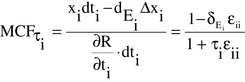 (3)
(3)
where ![]() is the proportional marginal external benefit generated by
xi. If the activity generates a positive externality, then
is the proportional marginal external benefit generated by
xi. If the activity generates a positive externality, then ![]() is positive
and the MCF is higher because taxing the commodity reduces the positive external
benefit from the commodity. If the
activity produces a harmful externality,
then
is positive
and the MCF is higher because taxing the commodity reduces the positive external
benefit from the commodity. If the
activity produces a harmful externality,
then ![]() is negative, and the MCF is lower, reflecting a social gain from reducing
a harmful externality when the commodity is taxed. Finally,
note that from the
above equation, the optimal tax rate on commodity i is the Pigouvian tax
is negative, and the MCF is lower, reflecting a social gain from reducing
a harmful externality when the commodity is taxed. Finally,
note that from the
above equation, the optimal tax rate on commodity i is the Pigouvian tax
![]() if
the government can levy lump-sum taxes and its MCF is one.
if
the government can levy lump-sum taxes and its MCF is one.
Public expenditure externalities
In the previous section, we showed how a distortion caused by an environmental externality, such as second hand smoking, can be incorporated in the formula for the MCF. There is another type of externality—which we will call a public expenditure externality—that operates through the government’s budget constraint. For example, an increase in cigarette consumption may drive up public expenditures on health care. Even in the absence of a “second-hand” smoke externality, smoking adversely affects non-smokers through the higher taxes that they have to pay as a result of higher public health care expenditures. The health care costs associated with smoking are often used to justify high taxes on tobacco products. Below, we show how these public expenditure effects can be incorporated in the formula for the MCF.
Suppose that the government provides a service, G, and the cost of providing this service is C(G, x) where ∂C/∂G > 0 is the marginal cost of providing the service and ∂C/∂x is the increase in the cost of providing a given level of service (say health care) as a result of an increase in the consumption of a private good x. For simplicity, we will ignore the taxes that are levied on other goods (that might be substitutes or complements with x), and therefore the public sector’s budget constraint requires that tx = C(G, x). Increasing the tax rate on x can increase the public sector’s net revenues either directly by increasing total revenues or indirectly by reducing net expenditures. Consequently, the MCF for taxing x will be equal to:
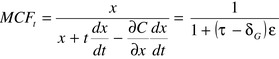 (4)
(4)
where it is assumed that the supply of the taxed commodity is perfectly
elastic so that dq/dt = 1 and ![]() which is the change in the cost of
public expenditures when individuals spend another dollar on x. When
which is the change in the cost of
public expenditures when individuals spend another dollar on x. When ![]() (e.g.
tobacco products), we see that the public expenditure effect reduces the MCF
when a higher tax rate reduces the demand for
the commodities that are
responsible for higher costs of providing a given level of public services. If
government could impose
lump-sum taxes, and the MCF was one, then the optimal
tax rate on x would be
(e.g.
tobacco products), we see that the public expenditure effect reduces the MCF
when a higher tax rate reduces the demand for
the commodities that are
responsible for higher costs of providing a given level of public services. If
government could impose
lump-sum taxes, and the MCF was one, then the optimal
tax rate on x would be![]() . In other words, the commodity would be taxed at a
rate that reflects its public expenditure externality, just as in the case of
the Pigouvian tax for a direct consumption externality.
. In other words, the commodity would be taxed at a
rate that reflects its public expenditure externality, just as in the case of
the Pigouvian tax for a direct consumption externality.
Addiction
Many individuals regret excessive consumption of some commodities, such as alcohol, tobacco and fatty foods. “For example, during 2000, 70 percent of current smokers expressed a desire to quit completely and 41 percent stopped smoking for at least one day in an attempt to quit, but only 4.7 percent successfully abstained for more than three months.”[4] Individuals who are prone to excessive drinking or smoking are said to have self-control or addiction problems. In many countries, excise taxes on alcohol and tobacco are viewed favourably as “sin taxes” because higher prices may reduce the degree of excessive consumption. See Badenes-Plá and Jones (2003) for a survey of the economics literature on addiction and taxes, Gruber and Kőszegi (2004) and Gruber and Mullainathan (2005) for recent empirical studies of the implications of addiction for efficiency and distributional effects of cigarette taxes, and the Economist (2006) for a discussion of public policies based on the “new paternalism”.
We use a simple model developed by O’Donoghue and Rabin (2006) to illustrate the way in which the self-control distortion can be incorporated in the evaluation of a tax increase on these commodities. Suppose an individual consumes only two goods, x1 and x2. The consumption of x2 provides constant marginal utility, normalized to equal one. The consumption of x1 provides the individual with a benefit V(x1) and also a psychic cost C(x1), which could be interpreted as a cost that arises from a future health problem. The individual make consumption decisions according to the following utility function:
![]() (5)
(5)
where Φ is a positive parameter. If Φ < 1, the individual is
said to have a self-control problem because he does not
take into account the
full personal cost consuming x1. The individual’s budget
constraint is q1x1 + x2 = I, where the price of
x2 is set equal to one. The individual consumes ![]() based on the first
order condition,
based on the first
order condition, ![]() .
.
However, the individual’s long-run happiness is based on the utility function:
![]() (6)
(6)
which fully reflects the cost that the individual incurs when he consumes
x1. The individual with self control problems over-consumes
x1 because the ideal consumption is based on ![]()
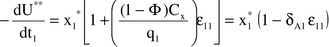
To evaluate the effects of a tax rate change, we will assume that the individual and society are concerned with the impact of the tax increase on the individual’s long-run utility. (See Bernheim and Rangel (2005) on using the individual’s long-term welfare in assessing policies.) The welfare effect of a tax increase is equal to:
![]() (7)
(7)
since, from the individual’s budget constraint,
dx2/dq1 = - ![]() -
q1dx1/dq1. Using the individual’s first
order condition, the following expression measures the harm caused by a tax
increase:
-
q1dx1/dq1. Using the individual’s first
order condition, the following expression measures the harm caused by a tax
increase:
 (8)
(8)
where ![]() = (dx1/dq1)(q1/x1) < 0 is
the price elasticity of demand for x1. The distortion caused by the
individual’s self-control problem is defined as:
= (dx1/dq1)(q1/x1) < 0 is
the price elasticity of demand for x1. The distortion caused by the
individual’s self-control problem is defined as:
![]() (9)
(9)
The ![]() parameter reflects the distortion that arises because there is a wedge
between marginal value of an additional unit of x to the individual
and its true
marginal cost. It can be interpreted as the neglected proportion of the
additional cost incurred in spending an additional dollar on x1. If
the individual has a self-control problem and Φ < 1,
parameter reflects the distortion that arises because there is a wedge
between marginal value of an additional unit of x to the individual
and its true
marginal cost. It can be interpreted as the neglected proportion of the
additional cost incurred in spending an additional dollar on x1. If
the individual has a self-control problem and Φ < 1, ![]() is
negative, and this factor tends to reduce the social harm from a tax increase.
Indeed, it is possible for a price increase to
make the individual better off,
at least as judged by his long-run utility function, if
is
negative, and this factor tends to reduce the social harm from a tax increase.
Indeed, it is possible for a price increase to
make the individual better off,
at least as judged by his long-run utility function, if ![]() and in this case, the
MCF would be a negative number. The formula for the marginal cost of public
funds for the commodity tax is:
and in this case, the
MCF would be a negative number. The formula for the marginal cost of public
funds for the commodity tax is:
![]() (10)
(10)
assuming that there are no other distortions in the economy. If the
government could raise revenue by imposing a lump-sum tax, such
that its MCF was
1.00, then the optimal tax rate on the commodity would be ![]() . The optimal sin tax
rate would reflect the neglected proportion of the additional cost
incurred in spending an additional dollar on x1. See
O’Donoghue, T. and M. Rabin (2006) for further discussion of optimal sin
taxes.
. The optimal sin tax
rate would reflect the neglected proportion of the additional cost
incurred in spending an additional dollar on x1. See
O’Donoghue, T. and M. Rabin (2006) for further discussion of optimal sin
taxes.
Obviously, incorporating these self-control distortions into the calculation of the MCF is controversial, but we think that lack of self-control problems, especially with regard to tobacco products, reflects public opinion and policy-makers’ views concerning the use of excise taxes. For this reason, we think that it is important to incorporate defective decision-making explicitly in the model so that it can be compared with the other distortions that affect the MCF. In this way, a better judgment can be made concerning the relative importance of self-control problems in the overall assessment of the appropriate level of excise taxation.
Market power
Suppose an excise tax is levied on a monopolist’s product. To keep the model as simple as possible, we will ignore all other tax and non-tax distortions in deriving an expression for the distortion due to monopoly power.
Let the after-tax profit of the monopolist be:
![]() (11)
(11)
where ![]() is the profit tax rate, and t is the per unit tax
rate.[5] Differentiating after-tax
profit with respect to the per unit tax rate, we obtain:
is the profit tax rate, and t is the per unit tax
rate.[5] Differentiating after-tax
profit with respect to the per unit tax rate, we obtain:
 (12)
(12)
where MC is the marginal cost of production. Ignoring distributional
effects, the indirect utility function for a representative
individual is
![]() .
The social welfare cost of an increase in the tax rate on the monopolist’s
product is:
.
The social welfare cost of an increase in the tax rate on the monopolist’s
product is:
 (13)
(13)
where ![]() is a measure of the distortion in the market caused by imperfectly
competitive behaviour,
is a measure of the distortion in the market caused by imperfectly
competitive behaviour, ![]() is the elasticity of demand for the
monopolist’s product,
is the elasticity of demand for the
monopolist’s product, ![]() is the marginal utility of income, and
is the marginal utility of income, and ![]() by
Roy’s Theorem. The first term in square brackets represents the net
increase in taxes paid by the private sector, given
that excise taxes are
deductible in computing the firm’s profit tax liability. The second term
represents the additional profit
tax that is paid as a result of the increase in
the price of the monopolist’s good. The third term is the reduction in
after-tax
profits sustained by the monopolist as a result of the decline in
output caused by the tax.
by
Roy’s Theorem. The first term in square brackets represents the net
increase in taxes paid by the private sector, given
that excise taxes are
deductible in computing the firm’s profit tax liability. The second term
represents the additional profit
tax that is paid as a result of the increase in
the price of the monopolist’s good. The third term is the reduction in
after-tax
profits sustained by the monopolist as a result of the decline in
output caused by the tax.
Total tax revenue is equal to ![]() Differentiating with respect to t
we obtain:
Differentiating with respect to t
we obtain:
 (14)
(14)
The first term in square brackets represents the net increase in tax
revenues, for a given level of output by the monopolist, the
second term is the
increase in profit tax revenues from the induced increase in the price of the
monopolist’s product, and
the third term is reduction in total tax
revenues from the reduction in the output produced by the monopolist. Note that
the government
sustains a reduction in profit taxes, ![]() as a result of the
reduction in the monopolist’s profit.
as a result of the
reduction in the monopolist’s profit.
From the above equations, we can obtain the following expression for the marginal cost of public funds from an excise tax levied on a monopolist’s product:
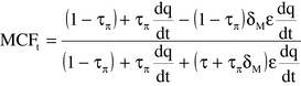 (15)
(15)
An interesting special case is where ![]() , which corresponds to a situation
where the monopoly is owned by the government and all of the profits and taxes
on the product are
received by the public treasury. This case is particularly
relevant for Thailand because of the Thai Tobacco Company, a state-owned
enterprise, has a monopoly on the sale and distribution of domestically produced
cigarettes in Thailand. In this situation, the
MCF is equal to:
, which corresponds to a situation
where the monopoly is owned by the government and all of the profits and taxes
on the product are
received by the public treasury. This case is particularly
relevant for Thailand because of the Thai Tobacco Company, a state-owned
enterprise, has a monopoly on the sale and distribution of domestically produced
cigarettes in Thailand. In this situation, the
MCF is equal to:
![]() (16)
(16)
which is independent of the degree of tax shifting. In this case, the total
tax rate on the product is effectively ![]() .
.
Smuggling
Norton (1988) has developed an economic model of smuggling and Usher (1986)
and Ray (1997, 380-384) have incorporated tax evasion
into the calculation of
the MCF. Below, we outline a simple model that incorporates smuggling into the
MCF for an excise tax. Suppose
the elasticity of the supply of the smuggled
commodity is ![]() . The price of the smuggled commodity will reflect
its production cost plus the smuggling costs that are incurred by the smugglers,
qs = p + cs. It will be assumed that these smuggling
costs are less than the per unit excise tax imposed on the legitimate goods.
Consumers
are willing to buy smuggled goods as long as the price of a smuggled
good plus the search costs, f, are less than the price of a
legitimate good
cigarette, qs = q – f. Assuming the excise
tax increases are fully reflected in the price of the legitimate good, this
implies that dq/dt
= dqs/dt = 1 if search costs are relatively
constant. The demand for the legitimate goods that are fully taxed is the
difference between
the total demand and the demand for smuggled goods or
xl = xT(q) –
xs(qs) where xT is the total number of
cigarettes consumed. The government’s tax revenue (ignoring all other
taxes) is R = txl. The marginal cost of public
funds from taxing cigarettes can then be expressed as:
. The price of the smuggled commodity will reflect
its production cost plus the smuggling costs that are incurred by the smugglers,
qs = p + cs. It will be assumed that these smuggling
costs are less than the per unit excise tax imposed on the legitimate goods.
Consumers
are willing to buy smuggled goods as long as the price of a smuggled
good plus the search costs, f, are less than the price of a
legitimate good
cigarette, qs = q – f. Assuming the excise
tax increases are fully reflected in the price of the legitimate good, this
implies that dq/dt
= dqs/dt = 1 if search costs are relatively
constant. The demand for the legitimate goods that are fully taxed is the
difference between
the total demand and the demand for smuggled goods or
xl = xT(q) –
xs(qs) where xT is the total number of
cigarettes consumed. The government’s tax revenue (ignoring all other
taxes) is R = txl. The marginal cost of public
funds from taxing cigarettes can then be expressed as:
 (17)
(17)
where v = xs/xT is the share of the smuggled goods in
total consumption and ![]() is the elasticity of demand for legitimate goods.
Smuggling increases the MCF because the tax base is smaller and the tax base is
more tax sensitive because smuggling gives individuals the opportunity to switch
to a non-taxed alternative. The elasticity of demand
for legitimate goods is
related to the elasticity of demand for total consumption and the smuggling
supply elasticity as follows:
is the elasticity of demand for legitimate goods.
Smuggling increases the MCF because the tax base is smaller and the tax base is
more tax sensitive because smuggling gives individuals the opportunity to switch
to a non-taxed alternative. The elasticity of demand
for legitimate goods is
related to the elasticity of demand for total consumption and the smuggling
supply elasticity as follows:
![]() where
(q/qs) = (p+cs+f)/(p+cs) <
where
(q/qs) = (p+cs+f)/(p+cs) < ![]() (18)
(18)
When the tax rate is raised, the volume of taxed goods decreases because total consumption falls and the volume of smuggled goods increases. For example, if 20 percent of the cigarettes are smuggled and if the elasticity of total demand for cigarettes is -0.40, the elasticity of demand for legitimate cigarettes could be as high as -0.813 if the elasticity of the supply of smuggled cigarettes is 0.50 and as much as -1.44 if the elasticity of the supply of smuggled cigarettes is 1.50. Therefore, ignoring the impact of smuggling by using the elasticity of total demand for cigarettes in the calculation of the MCF, rather then the elasticity of demand for legitimate cigarettes, may significantly under-estimate the MCF for cigarette taxes.
Distributional considerations
To this point, we have focused on the efficiency aspects of the marginal cost of public funds. However, all societies are concerned about the distributional impact of their tax system, and a tax increase that is borne mainly by the poor can be viewed as having a high social cost. Indeed, governments use distortionary taxes because of their concern for distributional equity, i.e. in the absence of these concerns, governments could simply rely on lump-sum taxes. Consequently, we need to incorporate distributional concerns in the measurement of the social marginal cost of public funds to fully evaluate tax and expenditure reforms.
To incorporate distributional considerations, we follow the procedure
developed by Feldstein (1972) and implemented by Ahmad and
Stern (1984) in the
analysis of commodity tax reform in
India.[6] Suppose there are H
households in the economy. Household h purchases ![]() units of commodity i at
the price qi. The household’s budget constraint is
units of commodity i at
the price qi. The household’s budget constraint is ![]() where
Ih is the household’s lump-sum income. The level of utility or
well-being that household h can obtain, given consumer and producer
prices, its
lump-sum income, its ownership of inputs, and its preferences, is indicated by
its indirect utility function,
Vh = Vh(q, Ih, G) where q
is the vector of consumer prices, p is the vector of producer prices, and G is a
vector of publicly-provided goods and
services. By Roy’s theorem,
∂Vh/∂qi = -λh
where
Ih is the household’s lump-sum income. The level of utility or
well-being that household h can obtain, given consumer and producer
prices, its
lump-sum income, its ownership of inputs, and its preferences, is indicated by
its indirect utility function,
Vh = Vh(q, Ih, G) where q
is the vector of consumer prices, p is the vector of producer prices, and G is a
vector of publicly-provided goods and
services. By Roy’s theorem,
∂Vh/∂qi = -λh![]() < 0 where λh(q, Ih, G) is the
household’s marginal utility of income and
< 0 where λh(q, Ih, G) is the
household’s marginal utility of income and ![]() (q, Ih,
G) is the household’s ordinary demand function for commodity i. The total
demand for commodity i is
(q, Ih,
G) is the household’s ordinary demand function for commodity i. The total
demand for commodity i is ![]() .
.
Suppose that tax and expenditure decisions are based on the social welfare function, S = S(V1, V2, ..., VH), which reflects the trade off that a society is willing to make when a policy makes some households better off and other household worse off. The distributional weight, βh = (∂S/∂Vh)λh, represents the value that the society places on an extra dollar of lump-sum income received by household h. It will be assumed that the social welfare function reflects a “pro-poor” preference such that βh is higher when Vh is lower.
The social valuation of the households’ welfare loss from an increase in the price of commodity i is:
![]() (19)
(19)
where ![]() is household h’s share of the total consumption of commodity i.
The ωi parameter is known as the distributional characteristic
commodity i, and it measures the social harm caused by increasing total
household
expenditure on xi by a dollar. Note that
ωi will tend to be larger when βh and
is household h’s share of the total consumption of commodity i.
The ωi parameter is known as the distributional characteristic
commodity i, and it measures the social harm caused by increasing total
household
expenditure on xi by a dollar. Note that
ωi will tend to be larger when βh and ![]() are
positively correlated. This means that ωi will be high for
commodities that are consumed mainly by the poor.
are
positively correlated. This means that ωi will be high for
commodities that are consumed mainly by the poor.
The social marginal cost of public funds from taxing commodity i can be defined as:
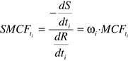 (20)
(20)
To compute the ωis, we need the βhs which reflect a society’s, or perhaps more accurately its policy-makers’, willingness to trade-off gains and losses sustained by different segments of society. The distributional weights are based on value judgments, and economists have no special insights into what constitutes the appropriate set of distributional weights. Economists, however, have tried to help policy-makers apply a consistent set of distributional weights. One approach is to use an explicit functional form for the relative distributional weights such as:
 (21)
(21)
where Yr is the income of a reference household (such as a household with the average income) and ξ ≥ 0 is a parameter that measures the society’s aversion to inequality. A standard normalization is to set βr = 1. If ξ = 0, βh = 1 for all h, and no consideration is given to distributional concerns. On the other hand, if Yh = 0.5 Yr, then βh = 1.414 if ξ = 0.5 and βh = 2 if ξ = 1. We use this approach to compute the SMCFs of the alcohol, tobacco, and fuel excise taxes.
The SMCF
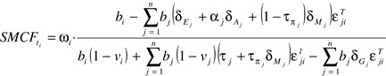
In the absence of a general equilibrium model to trace the effects of the
excise taxes on the prices of all commodities, we have assumed
that the excise
taxes on alcoholic beverages, tobacco, and fuel are fully reflected in their
product prices and that the prices of
other commodities are not affected.
Therefore, dqi/dti = 1 and dqj/dti
=0 for ![]() . Combining the tax and non-tax distortions discussed in the previous
section with the distributional characteristic of the taxed
good, we have the
following formula for the social marginal cost of funds for an excise tax:
. Combining the tax and non-tax distortions discussed in the previous
section with the distributional characteristic of the taxed
good, we have the
following formula for the social marginal cost of funds for an excise tax:
 (22)
(22)
Note that the components of the MCF that reflect the distortions are
multiplied by the ![]() s, which reflect the change in total demands for
goods, while the tax revenue changes (the second set of terms in the
denominator)
are multiplied by the elasticities of demand for legitimate
commodities, the
s, which reflect the change in total demands for
goods, while the tax revenue changes (the second set of terms in the
denominator)
are multiplied by the elasticities of demand for legitimate
commodities, the![]() s.
s.
PARAMETER VALUES
In this section, we describe how the various parameters used in the calculations were chosen.
Tax rates and budget shares
The tax rates and budget shares for the 10 commodity groups that were included in the analysis are shown in Table 1. The data used for calculating average tax rates are from the Ministry of Finance and National Economic and Social Development Board (NESDB). The statutory value-added tax was 7.0 percent in 2002, but the average tax rates are around 3.5 percent for most commodities except for food and clothing because some items and small firms are exempt from VAT. The average tax rates for alcoholic beverages and tobacco are 39.3 and 58.7 percent. Note that the tax rate for tobacco does not include the profit earned by the Thai Tobacco Monopoly (TTM), the state-owned company that has a monopoly in the production of domestic cigarettes. The average tax rate for fuel was 53.6 percent. An appendix describing the computations of the tax rates is available from the authors upon request. The budget shares were calculated from the aggregate consumption data from the NESDB. The budget share of alcohol was 4.2 percent, tobacco was 1.7 percent, and electricity and fuels was 2.4 percent of aggregate consumption spending in 2002.
TABLE 1: TAX RATES AND BUDGET SHARES FOR COMMODITIES IN THAILAND
|
Commodity
|
Tax Rate, τi
|
Budget Share, bi
|
|
1 Food
|
0.016
|
0.234
|
|
2 Alcohol
|
0.393
|
0.042
|
|
3 Tobacco
|
0.587
|
0.0.017
|
|
4 Clothing
|
0.0180
|
0.131
|
|
5 Health
|
0.035
|
0.064
|
|
6 Electricity and Fuels
|
0.536
|
0.024
|
|
7 Telecommunications
|
0.035
|
0.017
|
|
8 Housing and Water
|
0.036
|
0.126
|
|
9 Entertainment
|
0.037
|
0.042
|
|
10 Other Goods and Services
|
0.032
|
0.302
|
Demand elasticities
The estimated demand elasticities are shown in the matrix below. (The own-price elasticities are along the diagonal.)
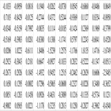
The price elasticities of demand for the ten commodities were estimated, using the Almost Ideal Demand System (AIDS) developed by Deaton and Muellbauer (1980), based on data on consumption expenditures from 1983 to 2002 in the Thailand National Income Account. The observations for 1998-99 were omitted because of the non-normal consumption shares in that year due to the economic crisis that began in the fall of 1997. (An appendix describing the demand estimation is available from the authors upon request.)
Our estimated own-price elasticity for alcoholic beverages is quite high, - 0.8429, compared to the -0.54 estimate obtained by Sarntisart (2003). However, it is less elastic than the values in the TDRI (2005) study where the price elasticities for color liquor, white liquor, imported liquor, beer and wine were -1.56, -2.73, -0.61, -2.68 and -0.60. Part of the reason for the differences in these estimates may be the fact that Sarntisart used household consumption data that included both tax and untaxed consumption while TDRI used the data from taxed consumption provided by the Excise Department. See Leung and Phelps (1993) and Badenes-Plá and Jones (2003, Table 3, p.140) for a summary of empirical estimates of the price elasticity of alcohol consumption in the US and other countries. These studies generally indicate that the demand for beer is relatively price insensitive (around -0.3) and the demand for spirits is price elastic (around -1.5) with the demand for wine having an intermediate price elasticity (around -1.00). Our estimate of the elasticity of the total demand for taxed alcohol falls within the usual range of estimates from other countries.
Our elasticity estimates indicate that alcohol is a gross complement for
tobacco (-0.5159) and for electricity and fuel (-0.3043)
while tobacco is a
very weak complement for alcohol (-0.0125), but a substitute for electricity and
fuel (0.2181).[7] Therefore an
alcohol tax rate increase will reduce the demand for both tobacco and fuel, and
therefore some of the increase in the
alcohol tax revenues from an alcohol tax
rate increase will be offset by declines in tobacco and fuel excise tax
revenues. (The
net effect on other commodity tax revenues is indeterminate, but
likely to be relatively small.) This negative effect on tobacco
and fuel excise
tax revenues will tend to raise the MCF for alcohol excise taxes. However, the
reductions in the consumption of
tobacco and fuel would also reduce the MCF for
alcohol excise taxes if the net distortion for these commodities, captured by
the
![]() terms in the MCF formula, are negative i.e. marginal social cost exceeds
marginal social benefit.
terms in the MCF formula, are negative i.e. marginal social cost exceeds
marginal social benefit.
The price elasticity for tobacco products is -0.7992, which is close to the -0.83 value obtained in a study by Pattamasiriwat (1989), but substantially higher than the -0.39 price elasticity found by Sarntisart (2003) based on household tobacco consumption data.[8] The differences may be due to smuggled or non-taxed cigarettes which the study by Sarntisart indicated are fairly prevalent in Thailand. (He found that about 46 percent of imported cigarette package littering in five provinces across Thailand were untaxed cigarette.) In other words, the price elasticity using data from the National Income Account is higher than for total household cigarette consumption, where taxed and untaxed cigarettes are included. Galbraith and Kaiserman (1997) found the same relationship in Canada where the price elasticity for taxed cigarettes was higher (-1.01) than that for total (taxed and untaxed) cigarette consumption (-0.4). Another study from Canada by Gruber, Sen and Stabile (2002) also found that the demand for taxed cigarettes was higher than the total demand (-0.70 versus -0.45). Our cross-price elasticities of demand imply that an increase in tobacco taxes will increase excise tax revenues from fuel, but increase distortion in the allocation of resources if there is a negative distortion in the market for fuel.
The demand for fuel and electricity consumption is quite price inelastic (-0.1833). Econometric studies of price elasticity of gasoline in the U.S. reviewed by Parry and Smart fall in the -0.3 to -0.90 range[9], and therefore our estimate of the own-price elasticity is considerably lower than that found in other countries. However, Wade (2003) showed that the short-run price elasticities of distillate fuel for residential and commercial uses were -0.15 and -0.13. In his review, he showed that short-run price elasticity of fuel oil for residential use in the U.S. was -0.10 to -0.59 and for commercial use was -0.07 to -0.19. Our econometric estimates indicate that electricity and fuel is a substitute for alcohol (0.5244) and a weak complement for cigarettes (-0.0185). Consequently, a fuel tax increase would tend to increase alcohol excise tax revenues and improve the allocation of resources if the net non-tax distortion in the alcohol market is positive.
Our demand estimation is based on the assumption that total consumer expenditure is exogenously determined. In particular, it assumes that variations in the prices of commodities do not affect labour supply decisions. Most of the previous studies of commodity tax reform such as Ahmad and Stern (1984) and Decoster and Schokkaert (1990) have either adopted this assumption or assumed separability between leisure and all other goods in consumers’ utility functions. These assumptions imply that in the absence of non-tax distortions the optimal commodity tax rate is a uniform tax rate because all good are equally “substitutable” with leisure, the non-taxed good.
Given the importance that the theoretical literature on optimal taxation has attached to the cross-price elasticities between leisure and commodities, it is important to briefly review the few papers have examined the empirical significance of the separability assumption for computing MCFs for commodity taxes. Madden (1995, p. 497), noting that several econometric studies of consumer demands and labour supplies reject the separability assumption, estimated models with and without the separability assumption, based on data for Ireland 1958-1988, and concluded that the MCF “rankings do not appear to be very sensitive to assumptions regarding separability between goods and leisure”. In particular, he found that the MCFs for alcohol, tobacco, and fuels were 1.664, 1.397, and 1.193, respectively, without imposing separability and 2.304, 1.504, and 1.418 when separability was imposed.[10] Although Madden’s estimates of the MCFs were higher when separability between leisure and commodities was imposed in estimating the demand elasticities, the rankings of the MCFs for the three commodities subject to high levels of excise taxation did not change. In his computations of the efficiency effects of excise taxes in the U.K., Parry (2003) assumed that petrol and alcoholic beverages were substitutes for leisure and that cigarettes were a complement. However, the implied cross-price elasticities between leisure and the price of these commodities were very low and did not have a material effect on Parry’s measures of the marginal excess burdens imposed by the excise taxes.[11]
In marked contrast with the above studies, West and Williams (2006) found that including the cross-price effect between labour supply and the price of gasoline had a significant effect on the magnitude of the MCF for the excise tax on gasoline in the United States. They estimated a model based on individual household’s expenditures gasoline and all other goods and their labour income, and found that higher gasoline prices increased labour income (reduced the demand for leisure). This reduced the MCF from taxing gasoline and increased the optimal gasoline tax rate. However, only one of the three cross-price elasticity between labour income and the price of gasoline that they estimated was significantly different from zero (males in households with two adults) and that point elasticity was very low 0.013.
The West and Williams results are somewhat surprising, and the importance of the cross-price effects between excise taxes and labour supplies need to be investigated more completely. Given our current and very limited knowledge about the importance of these effects, we have proceeded by adopting the conventional assumption that these effects do not have a material effect on the rankings of the MCFs for excise taxes.
Environmental externalities
In spite of a significant body of research, there is a great deal of
uncertainty regarding the appropriate values to use for the ![]() parameters
for developed countries, such as the United States or the United Kingdom. There
is even greater uncertainty for a developing
country, such as Thailand, where
much less empirical research has been done on the environmental impacts of
alcohol, tobacco, and
fuels and where economic, social, and environmental
conditions may be substantially different than in the developed countries.
Nonetheless,
we have had to make some choices regarding these parameters, which
are shown in Table 2. A detailed description of the benchmark
parameter values
is given in the following sections of this
paper.[12]
parameters
for developed countries, such as the United States or the United Kingdom. There
is even greater uncertainty for a developing
country, such as Thailand, where
much less empirical research has been done on the environmental impacts of
alcohol, tobacco, and
fuels and where economic, social, and environmental
conditions may be substantially different than in the developed countries.
Nonetheless,
we have had to make some choices regarding these parameters, which
are shown in Table 2. A detailed description of the benchmark
parameter values
is given in the following sections of this
paper.[12]
TABLE 2: PARAMETER VALUES FOR NON-TAX DISTORTIONS
|
|
Low Case
|
Benchmark Case
|
High Case
|
|
|
Environmental Externality,
|
||
|
Alcohol
|
-0.007
|
-0.014
|
-0.05
|
|
Cigarettes
|
0
|
-0.025
|
-0.05
|
|
Fuel
|
-0.05
|
-0.10
|
-0.38
|
|
|
Public Expenditure Externality,
|
||
|
Alcohol
|
0.001
|
0.002
|
0.008
|
|
Cigarettes
|
0.004
|
0.05
|
0.30
|
|
Fuel
|
0.09
|
0.18
|
0.27
|
|
|
Addiction,
|
||
|
Alcohol
|
-0.03, 0.017
|
-0.06, 0.052
|
-0.12, 0.071
|
|
Cigarettes
|
-0.8, 0.18
|
-1.65, 0.18
|
-3.3, 0.18
|
|
Fuel
|
0, 0
|
0, 0
|
0, 0
|
|
|
Market Power,
|
||
|
Alcohol
|
0.065
|
0.13,
|
0.26
|
|
Cigarettes
|
0.10
|
0.20
|
0.30
|
|
Fuel
|
0
|
0
|
0
|
|
Telecom
|
0.10
|
0.25
|
0.55
|
|
|
Net Non-Tax Distortion: δE -
δG + αδA + (1 -
τπ)δM
|
||
|
Alcohol
|
0.037
|
0.072
|
0.115
|
|
Cigarettes
|
-0.148
|
-0.372
|
-0.944
|
|
Fuel
|
-0.140
|
-0.280
|
-0.65
|
|
Telecom
|
0.070
|
0.175
|
0.385
|
|
|
Smuggling,
|
||
|
Alcohol
|
-0.54, 0.080
|
-0.54, 0.160
|
-0.54, 0.240
|
|
Cigarettes
|
-0.40, 0.023
|
-0.40, 0.155
|
-0.40, 0.300
|
|
Fuel
|
Na
|
na
|
na
|
Our estimates for the “environmental” externalities from alcohol
are based on Smith (2005)’s recent survey of alcohol
excise taxes because
he decomposed these externalities in a way that is consistent with our
framework.[13] Smith estimated that
the total externality cost of alcohol in the U.K. is 17 percent of the pre-tax
price. Based on his breakdown
of the social costs of alcohol, we have
decomposed his total externality into an 8.2 percent private sector
“environmental”
externality (losses sustained by employers etc.), a
1.31 percent public expenditure externality (health costs, crime, and social
responses) and 7.3 percent “internality” from unemployment and
pre-mature death. (The latter is included in the ![]() parameter for alcohol
to be discussed in Section 3.6.) The δE parameter for the
benchmark case was calculated as -0.082*(1–0.393)*0.27 =
-0.014. The 0.393 is the tax rate on alcohol
in Thailand. We multiply by (1
– 0.393) to express the externality as a percentage of the tax inclusive
price. We then multiply
by the 0.27 which is the ratio of the purchasing power
parity Thai GDP per capita to the U.K GDP per
capita.[14] The High Case is the
benchmark case without the adjustment for the relative GDPs in Thailand and the
U.K. The Low Case is 50 percent
of the benchmark case.
parameter for alcohol
to be discussed in Section 3.6.) The δE parameter for the
benchmark case was calculated as -0.082*(1–0.393)*0.27 =
-0.014. The 0.393 is the tax rate on alcohol
in Thailand. We multiply by (1
– 0.393) to express the externality as a percentage of the tax inclusive
price. We then multiply
by the 0.27 which is the ratio of the purchasing power
parity Thai GDP per capita to the U.K GDP per
capita.[14] The High Case is the
benchmark case without the adjustment for the relative GDPs in Thailand and the
U.K. The Low Case is 50 percent
of the benchmark case.
The environmental externality from tobacco is mainly second-hand smoke, and we do not know of any estimates for this type of externality. As noted in the literature, much of the second-hand smoke problem occurs within the family, and therefore it is debatable whether this is an “externality”. The incidence of second-hand smoke in Thailand has also been reduced with non-smoking in public transit, schools and public offices, but smoking is still permitted in bars and non air-conditioned restaurants in Thailand. Overall, we think that the second-hand smoke externality is likely to be small (not many people offer to pay smokers to butt out their cigarettes), but obviously this is controversial and based on a value judgment that we admit is difficult to defend.
Newbery’s (2005) estimate of the environmental cost is 14 pence per litre for gasoline in UK, excluding road costs which we treat as a public expenditure externality, and including 3.2 pence per litre for accidents. Our benchmark value for fuel environmental externality is -(0.14£/litre)(67.8B/£)(0.27)(25B/litre) = -0.10 using the relative Thai to UK GDP per capita to is 27 percent of the U.K GDP per capita. For the High Case, we do not adjust for differences in Thai to UK real GDP per capita -(0.14£/litre)(67.8B/£)/(25B/litre) = -0.38. The Low Case is 50 percent of the Benchmark case.
Public expenditure externalities
As is widely recognized, alcohol, tobacco and fuel consumption may directly or indirectly drive up public expenditures, forcing taxpayers to pay higher taxes to finance them or crowding out other valuable public services. This distortion operates through the government’s budget constraint, and therefore it has a distinct effect on the marginal cost of public funds, even though most studies do not distinguish between environmental externalities and public expenditure externalities.
The public expenditure externality for alcohol is based on an estimate of 1.3 percent of the pre-tax price in the U.K by Smith (2005). The distortion parameter was calculated as 0.013*(1 – 0.393)*0.27 = 0.002 where, as before, we multiply by (1 – 0.393) to express the externality as a percentage of the tax inclusive price. We then multiply by the 0.27, which is the ratio of the purchasing power parity Thai GDP per capita to the U.K GDP per capita. The High Case is the Benchmark Case without the adjustment for the relative GDPs in Thailand and the U.K. The Low Case is 50 percent of the benchmark case.
The benchmark value for the impact of smoking on health care costs uses the
estimates from Manning et al. (1989) of $US 0.25 per package
(figures updated to
2003) See Cnossen (2005, p.37). This value was multiplied by 0.20 to reflect
the relative GDP in Thailand and
divided by 1.08, the price of a package of
cigarettes in Thailand. The resulting estimate of the ![]() parameter is
(0.25)(0.20)/(1.08)= 0.046, rounded to 0.05. The High Case was obtained using
the position expressed by the Director-General
for WHO, Dr. Lee Jong-wook, that
15 percent of all health care costs in high income countries are due to smoking.
Public health care
costs are two-thirds of total health care costs in Thailand.
Total health care costs in 2002 were 333,798 million Baht and total
value of
cigarette consumption was 55,832 million Baht. Therefore the High Case
parameter value was calculated as (0.32)(0.15)(333,3798)/(45,219)
= 0.29,
rounded to 0.30. The Low Case parameter value was based on the Sarntisart
(2003, p. 43) estimate that the direct health
care costs of tobacco were 249
million Baht in 2003. This would imply that the
parameter is
(0.25)(0.20)/(1.08)= 0.046, rounded to 0.05. The High Case was obtained using
the position expressed by the Director-General
for WHO, Dr. Lee Jong-wook, that
15 percent of all health care costs in high income countries are due to smoking.
Public health care
costs are two-thirds of total health care costs in Thailand.
Total health care costs in 2002 were 333,798 million Baht and total
value of
cigarette consumption was 55,832 million Baht. Therefore the High Case
parameter value was calculated as (0.32)(0.15)(333,3798)/(45,219)
= 0.29,
rounded to 0.30. The Low Case parameter value was based on the Sarntisart
(2003, p. 43) estimate that the direct health
care costs of tobacco were 249
million Baht in 2003. This would imply that the ![]() parameter would be
(249)/(55,832)= 0.004.
parameter would be
(249)/(55,832)= 0.004.
Newbery’s (2005) estimate of road costs are 25.2 pence/litre in the U.K. The benchmark value for fuel public expenditure externality is (0.252£/litre)(67.8Baht/£) (0.27)(25Baht/litre) = 0.18. The High Case is 50 percent higher and the Low Case is 50 percent lower that the Benchmark Case.
Addiction
As noted in the introduction, excise taxes are often viewed as “sin taxes”, levied in order to discourage the consumption of products that are “bad for people”. In Section 2.3, we used the O’Donoghue and Rabin (2006) model to formalize the view that some individuals engage in excessive consumption of alcohol and tobacco because of defective decision-making. Obviously, the choice of the parameters is difficult in the absence of empirical research that might shed light on the degree of excessive consumption. Some progress in this direction has made with the study by Gruber and Mullainathan (2005) which suggested that cigarette taxes in the U.S. and Canada might make some individuals better off by inducing them to quit smoking, or at least reduce their consumption of cigarettes. More research on this topic is obviously needed before anyone can feel fully comfortable in incorporating addiction in the MCF calculations. However, strong views about addiction dominate public views about the importance of excise taxes on alcohol and tobacco. We hope that our formalization of these views will help to assess their importance relative to the other factors, such as externalities, market power, and smuggling, which also influence public policy regarding excise taxes.
The calculation of the addiction parameter was based on Smith’s estimate that the income loss from unemployment and premature death in the U.K. was 7.3 percent of the pre-tax price of alcohol. The value of value Cx/qx was calculated as
(0.073*(1-0.373)*0.27)/(0.05) = 0.24. (The division by 0.05 represents the calculation of the present value of the annual stream of lost income at a five percent discount rate.) Gruber and Kőszegi (2004, Table 2, page 1977) used values of Φ = 0.60 to Φ = 0.9 to reflect hyperbolic discounting of future costs and benefits by individuals with addiction problems. We use the mid-range value of 0.75. This implies that our benchmark parameter value for δA for alcohol is (0.75-1)0.24 = -0.06. The Low Case is 50% of the benchmark case and the High Case is twice the benchmark case. The proportion of the population addicted to alcohol, α, is the 3.34 percent of the population who reportedly drink every day plus 50 percent of the 3.79 percent who drink 3 to 4 times per week.[15] Thus the Benchmark figure for α is 3.34+(0.5)3.79 = 5.2 percent. The High Case figure is 3.34 + 3.79 = 7.1 percent. The Low Case figure is half the percentage that drinks every day.
The Benchmark value for the addiction distortion for cigarettes was obtained
using Gruber and Kőszegi’s (2004, p.1979)
estimate that the cost in
terms of life years lost per pack of cigarettes in the United States is $35.64.
The purchasing power equivalent
per capita GDP in Thailand is 20 percent of the
U.S. and price of cigarettes in Thailand in U.S. is 1.08. See Guindon, Tobin
and
Yach (2002). We also used a value of 0.75 for ![]() as in the alcohol
addiction calculations. Taken together, our benchmark value for
δA for cigarettes is (0.75-1)(35.64/1.08)(0.20) = -1.65,
implying that the “neglected cost” per package of cigarettes in
Thailand is 165 percent of the actual price. The Low Case is 50% of the
Benchmark Case and the High Case is twice the Benchmark
Case. The estimate for
the proportion of addicted smokers is the 18 percent of Thais who are reported
to be regular smokers.[16]
as in the alcohol
addiction calculations. Taken together, our benchmark value for
δA for cigarettes is (0.75-1)(35.64/1.08)(0.20) = -1.65,
implying that the “neglected cost” per package of cigarettes in
Thailand is 165 percent of the actual price. The Low Case is 50% of the
Benchmark Case and the High Case is twice the Benchmark
Case. The estimate for
the proportion of addicted smokers is the 18 percent of Thais who are reported
to be regular smokers.[16]
Market power
Imperfect competition is a market distortion, but it has played little role in the discussion of excise tax policy, even though in beer and tobacco markets are highly concentrated in many countries.[17] For example, Cnossen and Smart (2005) do not discuss the implications of firms’ market power for setting cigarette taxes. In our calculation, we incorporate a measure of the distortion caused by market power in the beer and white whiskey market, the tobacco market, and the mobile phone market in Thailand. The latter is included, even though an excise tax was not levied on telecommunication services in 2002 because excise tax increases on alcohol, tobacco, and fuels might increase (decrease) the demand for telecommunication services leading to an improvement (deterioration) in resource allocation.
The domestic beer market in Thailand is dominated by two large firms—Boon Rawd Brewery Co. and Thai Beverage PLC. In 2002, Thai Beverage PLC had 65 percent of the beer market and Boon Rawd Brewery Co. had 26 percent. Thai Beverage PLC also has a monopoly power over the white liquor market.[18]
The market power parameter for alcohol was based on the assumption that the sale of beer and white liquor, which represent approximately 70 percent of total alcohol sales, is a Cournot duopoly. Therefore, δM = 0.5(1/-2.7)0.70 = 0.13 where the 0.5 is one divided by the number of firms and -2.7 is an estimate of the elasticity of demand for beer and white liquor from the study by TDRI (2005).[19] This calculation implies that the firms earn a pure profit margin of 13 percent. The High Case is twice the Benchmark Case and the Low Case is 50 percent of the Benchmark Case. It is assumed that marginal changes in pure profits are taxed at the statutory Thai corporate income tax rate of 30 percent. Our analysis is based on the assumption that excise taxes are fully shifted to consumers. However, a study by Young and Bielińska-Kwapisz (2002) indicates that taxes on beer and spirits are over-shifted in the United States. In their study, taxes on beer and spirits increased consumer prices by approximately 1.7 times the tax rate. We also briefly consider the impact of the over-shifting of alcohol excise taxes on the MCF for alcohol.
The Thai Tobacco Monopoly (TTM) has a monopoly in production of domestic
brands. The market power distortion in the Benchmark Case,
![]() , is based
on an estimate of the market power of European tobacco companies from a study by
Delipalla and O’Donnell
(2001).[20] We have assumed that
all of the profits of the TTM go to the Thai government, or
, is based
on an estimate of the market power of European tobacco companies from a study by
Delipalla and O’Donnell
(2001).[20] We have assumed that
all of the profits of the TTM go to the Thai government, or![]() . Therefore, the total
effective tax rate on cigarettes in the benchmark case is 0.587 + 0.20 = 0.79,
which is very close to the
effective tax rate that Sarntisart (2003, p.43) used
in his study of tobacco control in Thailand. The High Case is twice the
benchmark
case and the Low Case is half the benchmark case.
. Therefore, the total
effective tax rate on cigarettes in the benchmark case is 0.587 + 0.20 = 0.79,
which is very close to the
effective tax rate that Sarntisart (2003, p.43) used
in his study of tobacco control in Thailand. The High Case is twice the
benchmark
case and the Low Case is half the benchmark case.
The mobile phone market in Thailand is dominated by two large firms —Advance Info Service PLC and Total Access Communication PLC. In the absence of other information about the degree of market power exercised by these firms, we have assumed that the δM is 0.25 in the Benchmark case, 0.55 in the High Case, and 0.10 in the Low Case.[21]
Table 2 also shows the net non-tax distortions, created by the environmental and public expenditure externalities, addiction, and market power. For the Benchmark parameter values, the positive values for alcohol and telecommunications imply that the market price exceeds the net social cost and an increase in output would produce a net social gain. Therefore, a tax increase that reduces the consumption of these commodities will produce high efficiency loss because of the under-provision of these commodities. The negative values for tobacco and fuel imply that the marginal social costs of these commodities exceed their consumer price and a reduction in the consumption of these goods produces a net social gain. Thus the net non-tax distortions tend to lower the MCFs for these commodities. Of course, the tax distortions, exacerbated by smuggling, also affect the MCFs, and we consider this source of distortion below.
Smuggling
To capture the effect of alcohol smuggling, we use a total demand elasticity
of ![]() based on the estimate of the demand for alcohol in Sarntisart (2003). A
study of alcohol smuggling in Thailand by TDRI (2006) indicates
that illegally
produced and smuggled alcohol is about 16 percent of alcohol consumption.
[22] For the Low Case, we use 8 percent
and for the High Case we use 24 percent.
based on the estimate of the demand for alcohol in Sarntisart (2003). A
study of alcohol smuggling in Thailand by TDRI (2006) indicates
that illegally
produced and smuggled alcohol is about 16 percent of alcohol consumption.
[22] For the Low Case, we use 8 percent
and for the High Case we use 24 percent.
To capture the effect of tobacco smuggling, we use a total demand elasticity
of ![]() based on this widely used value of the elasticity of demand for
cigarettes. The Benchmark value for the proportion of smuggled
cigarettes is
from a survey by Sarntisart (2003. p.26) who found that “15.5% of their
cigarettes packages had warning labels
in English or other non-Thai languages or
no warning labels, and were probably illegally imported”. The Low Case
estimate
was based on the results of a different survey, also described in
Sarntisart (2003), where it was found that 46 percent of discarded
imported
cigarette packages had warning label in wrong language or no warning labels.
Given that imports represent 4.89 percent
of total consumption of cigarettes,
the proportion of smuggled cigarettes in the Low Case was calculated as
0.46(4.89) = 2.22 percent.
(The share of imported cigarettes was based on
figures in Sarntisart (2003 Table 3.4 p. 9).) The High Case figure is twice the
Benchmark figure.
based on this widely used value of the elasticity of demand for
cigarettes. The Benchmark value for the proportion of smuggled
cigarettes is
from a survey by Sarntisart (2003. p.26) who found that “15.5% of their
cigarettes packages had warning labels
in English or other non-Thai languages or
no warning labels, and were probably illegally imported”. The Low Case
estimate
was based on the results of a different survey, also described in
Sarntisart (2003), where it was found that 46 percent of discarded
imported
cigarette packages had warning label in wrong language or no warning labels.
Given that imports represent 4.89 percent
of total consumption of cigarettes,
the proportion of smuggled cigarettes in the Low Case was calculated as
0.46(4.89) = 2.22 percent.
(The share of imported cigarettes was based on
figures in Sarntisart (2003 Table 3.4 p. 9).) The High Case figure is twice the
Benchmark figure.
CALCULATIONS OF THE MCFS
The calculations of the MCFs for the Benchmark parameter values are shown in Table 3. Alcohol taxes have the highest MCF at 2.312, followed by tobacco at 2.187, and fuels at 0.532. The large gaps between the MCFs for alcohol and tobacco and the MCF for fuels indicates that there would be a substantial welfare gain from a revenue neutral tax reform which reduced tax rates on alcohol and tobacco and increased the tax rate on fuel. However, this conclusion has to be tempered by the fact that the low MCF for fuel is likely due to our low estimate of the elasticity of demand for fuel—the elasticity of demand is one-quarter that of alcohol and tobacco.
TABLE 3: MCFS FOR EXCISE TAXES AND THE VAT: BENCHMARK PARAMETER VALUES
|
|
Excise Tax
on Alcohol
|
Excise Tax on Tobacco
|
Excise Tax on Fuel
|
VAT
|
|
MCFs
|
2.312
|
2.187
|
0.532
|
1.080
|
|
Contribution of Non-Tax Distortions to the MCFs:a
|
|
|
|
|
|
Environmental Externalities,
|
-0.075
|
0.052
|
-0.004
|
-0.004
|
|
Public Expenditure Externalities,
|
-0.275
|
0.182
|
-0.012
|
-0.007
|
|
Market Power,
|
0.335
|
0.457
|
-0.212
|
-0.005
|
|
Addiction,
|
-0.156
|
-0.298
|
-0.0007
|
-0.012
|
|
Smuggling
|
0.323
|
0.618
|
0.022
|
0.019
|
|
MCFs in the Absence of Non-Tax Distortions
|
1.985
|
1.566
|
0.737
|
|
|
MCFs in the Absence of Non-Tax Distortions and Interactions with Other
Tax Bases
|
1.496
|
1.882
|
1.109
|
|
aA positive (negative) value means that the factor increases (reduces) the MCF.
Although the excise taxes are the focus of our analysis, we have also calculated the MCF for a VAT increase, based on the assumption that the VAT increase would be fully reflected in the prices of alcohol, cigarettes, and fuel and increase the prices of the other expenditure categories to the same degree that their current effective tax rates reflect the VAT. Thus, for example, we assume that food, clothing, and housing would increase by 0.23, 0.251 and 0.506 percentage points from a one percent VAT increase because of zero rating and exemptions. The MCF for the VAT increase with the Benchmark parameter values was 1.080, much lower than the MCFs for alcohol and cigarette excise taxes, but higher than for the fuel excise tax. It should be borne in mind that the VAT increase is similar (although not exactly equivalent) to a proportional wage tax increase because it reduces workers’ real wage rates. Our relatively low estimate for MCFVAT reflects our assumption of fixed labour supplies. However, a computations of the MCF for an income tax increase in Thailand in the mid-1990s by Poapangsakorn et al. (2000, Table 6, p.76) were in the 1.04 to 1.11 range, and therefore comparable to our estimate of the MCF for a VAT increase.
Our main contribution to the calculation of MCFs for commodity taxes is that
we have incorporated most of the key factors that affect
decisions or attitudes
concerning excise taxes—environmental externalities, public expenditure
externalities, imperfect competition,
addiction, smuggling and the interactions
of tax bases—in a single model. In Table 3, we show how each of these
distortions
affects the MCFs for alcohol, tobacco and fuel. To assess the
contribution of each distortion to the MCFs, we set each one in turn
equal to
zero and then recalculated the MCFs. For example, our calculations indicated
that if all environmental externalities were
ignored, the MCF for alcohol would
have been 2.387 instead of 2.312. Therefore, incorporating the environmental
externalities at
the Benchmark parameter values reduced the MCF for alcohol by
0.075. Similarly, environmental externalities increased the MCF for
tobacco
taxes by 0.052. This may seem surprising, but it can be explained by the fact
that the ![]() for tobacco is quite low and an increase in tobacco taxes would increase
the demand for fuels (with a cross-price elasticity of 0.218)
where
for tobacco is quite low and an increase in tobacco taxes would increase
the demand for fuels (with a cross-price elasticity of 0.218)
where ![]() parameter is
four times larger (in absolute value). Similarly, incorporating the public
expenditure externalities reduces the MCF
for alcohol taxes by 0.275, but
increases the MCF for cigarette taxes by 0.182.
parameter is
four times larger (in absolute value). Similarly, incorporating the public
expenditure externalities reduces the MCF
for alcohol taxes by 0.275, but
increases the MCF for cigarette taxes by 0.182.
The market power distortion raises the MCFs for alcohol and tobacco by 0.335 and 0.457 respectively, but lowers the MCF for fuel by 0.212, even though the fuel industry is assumed to be competitive. The reason for the reduction in the MCF for fuel is that a fuel tax increase raises the demand for alcohol (with a cross-price elasticity of 0.524), and this helps to offset the alcohol market power distortion.
As might be expected, incorporating addiction significantly reduces the MCFs for excise taxes on alcohol and cigarettes. The 0.298 reduction in the MCF for cigarettes is relatively large because addicted smokers are assumed to ignore costs of smoking that are 165 percent of the product price in our Benchmark Case. However, smuggling has an even greater impact on the MCFs for alcohol and tobacco, raising them by 0.323 and 0.618 respectively, i.e. the impact of smuggling more than offsets the impact of addiction on the MCFs. The second last row in Table 3 shows the MCFs in the absence of the non-tax distortions (including smuggling). These calculations indicate that the combined effect of the non-tax distortions and smuggling increase the MCFs for alcohol and tobacco excises, but reduces the MCF for fuel taxes.
The last row of Table 3 shows how the MCF is affected by a failure to account for the effect of an excise tax rate change on tax revenues from other tax bases. (Most discussions of tobacco taxation, such as Sunley et al. (2000, Table 17.5, p.423), only focus on the effect of a tobacco tax increase on tobacco tax revenues and ignore the effects on other sources of tax revenue.) Our calculations show that incorporating the effects on other tax revenue sources is very important in evaluating an alcohol excise increase. The MCF for alcohol would be significantly underestimated if we ignore the effects of an alcohol tax rate increase on the revenues from other commodity taxes. Recall that our demand estimation indicates that alcohol is a complement for both tobacco and fuel, with cross-price elasticities of -0.516 and -0.304 respectively. Increasing the alcohol excise tax reduces revenues for these other two heavily taxed commodities, and this account in part for alcohol’s relatively high MCF. Conversely, incorporating the interactions with the other tax bases lowers the MCFs for tobacco and fuel taxes.
Our computations in Table 3 are based on the assumption that excise taxes are fully reflected in consumer prices. However, in imperfectly competitive markets, taxes may be under-shifted or over-shifted even if the marginal cost of production is constant in the long-run. As previously noted, Young and Bielińska–Kwapisz (2002) found that beer and spirit prices in the United States increased by about $1.70 for a $1.00 excise tax increase. If the same degree of over-shifting of the alcohol excise taxes occurs in Thailand, then the MCF for the alcohol excise tax would be 8.927, making it an extremely expensive source of tax revenue. The sensitivity of the calculation of the MCFs to the degree of tax shifting indicates that future research should try to determine the degree to which excise taxes are over or under-shifted in imperfectly competitive markets.
To summarize, our analysis indicates that smuggling, market power, and addiction have potentially large impacts on the MCFs, especially for tobacco taxes, and that interactions with other tax bases is especially important for calculating the MCFs for excise taxes.
These conclusions are based on a particular set of parameter values. To determine the sensitivity of our results to the choice of the parameter values, we recalculated the MCFs using the High Case and Low Case values for the parameters. Table 4 indicates that the MCFs are lower in the High Case. This means that the higher parameter values for the environmental and public expenditure externalities and addiction more than offset the use of the higher parameter values for market power and smuggling. The contributions of the various distortions to the MCFs are also generally larger (in absolute value) than in the Benchmark case. The only major anomaly is that the public expenditure externality now reduces the MCF for tobacco.
TABLE 4: MCFS FOR EXCISE TAXES AND THE VAT: HIGH DISTORTION CASE
|
|
Excise Tax on Alcohol
|
Excise Tax on Cigarettes
|
Excise Tax on Fuel
|
VAT
|
|
MCFs
|
1.95
|
2.10
|
0.32
|
1.05
|
|
Contributions of Non-Tax Distortions to the MCFs:a
|
|
|
|
|
|
Environmental Externalities,
|
-0.243
|
0.257
|
-0.016
|
-0.012
|
|
Public Expenditure Externalities,
|
-0.725
|
-0.220
|
-0.010
|
-0.021
|
|
Market Power,
|
0.388
|
0.442
|
-0.424
|
-0.004
|
|
Addiction,
|
-0.304
|
-0.629
|
0.00006
|
-0.024
|
|
Smuggling
|
0.269
|
1.178
|
0.019
|
0.031
|
aA positive (negative) value means that the factor increases (reduces) the MCF.
Table 5 shows similar calculations for the Low Case parameters values. The MCFs for alcohol and tobacco are lower than in the Benchmark case, but the MCF for fuels increases from 0.532 to 0.645. Thus the rankings of the MCFs for the three excise taxes are the same in the Benchmark and Low Cases, but rankings of alcohol and tobacco are reversed in the High Case.
TABLE 5: MCFS FOR EXCISE TAXES AND THE VAT: LOW DISTORTION CASE
|
|
Excise Tax on Alcohol
|
Excise Tax on Cigarettes
|
Excise Tax on Fuel
|
VAT
|
|
MCFs
|
2.220
|
1.794
|
0.645
|
1.083
|
|
Contributions of Distortions to MCF:a
|
|
|
|
|
|
Environmental Externalities,
|
-0.028
|
0.029
|
-0.002
|
-0.001
|
|
Public Expenditure Externalities,
|
-0.090
|
0.086
|
-0.007
|
-0.003
|
|
Market Power,
|
0.182
|
0.200
|
-0.095
|
0.004
|
|
Addiction,
|
-0.069
|
-0.109
|
-0.001
|
-0.006
|
|
Smuggling
|
0.198
|
0.142
|
0.014
|
0.009
|
aA positive (negative) value means that the factor increases (reduces) the MCF.
The large gap between the MCFs for the excise taxes on alcohol and cigarettes and the MCF for the fuel excise tax indicates that there is a potentially large efficiency gain from a revenue-neutral tax reform that would increase the fuel excise tax and reduce the excise taxes on alcohol and cigarettes. We can give an indication of the potential size of these gains by considering small cuts in the alcohol and cigarette excise taxes, offset by a revenue-neutral increase in the fuel excise tax. The gains and losses from these tax revenue changes can be evaluated at the average of the pre-reform and post-reform MCFs and compared to the total increase in fuel tax revenue. For example, using the Benchmark parameter values, the fuel excise tax would have to be raised by a 0.688 percentage point to maintain revenues if the excise taxes on alcohol and tobacco were each cut by one percentage point. This revenue-neutral tax reform would increase the MCF for the fuel excise tax from 0.532 to 0.536 and lower the MCFs for alcohol and tobacco excises from 2.312 to 2.269 and from 2.187 to 2.137 respectively. Evaluated at the average of the pre-reform and post-reform MCFs, there would be a net efficiency gain of 1.72 Baht for each additional Baht of fuel tax revenue collected. One limitation of our approach is that does not allow us to determine how large the revenue-neutral fuel tax increase should be to maximize the net efficiency gain from this type of excise tax reform.
CALCULATIONS OF THE SMCFS
To calculate the distributionally-weighted MCFs for the three excise taxes, we have computed the βs using (21) and using a fairly conventional range of values for ξ, 0.25 to 1.00. The average per capita monthly income in Thailand of 3,844 Baht in 2002 was used as the reference income level.[23] Figure 1 shows the distributional weights at the average income levels in the 10 deciles. The distributional weights range between 1.572 and 6.114 at the average income in the first decile, 629 Baht per month, and between 0.708 and 0.252 at the average income level in the 10th decile, 15,256 Baht per month, when the values of ξ range between 0.25 and 1.00. To compute the distributional characteristics of the commodities, we have used the expenditure patterns of 90 household groups (based on data from five urban areas and four rural regions in each decile) from the Socio-Economic Survey (SES) 2002. Table 6 shows the computed distributional characteristics for all of the commodities for values of ξ between 0.25 and 1.00, normalized so that the distributional characteristic for food is equal to one. Note that when ξ = 0.25, alcohol, tobacco and fuel have almost identical distributional characteristic values, around 0.88. Therefore, with a moderate set of distributional weights, the relative SMCFs are the same as their efficiency components, the MCFs. Divergences in the distributional characteristics appear when larger values of ξ are used. Among the three commodities subject to the excise taxes, tobacco has the lowest ω. Electricity and fuels has the highest when ξ = 0.50 and alcohol has the highest when ξ = 1.00. Therefore, the relative ranking of the distributional characteristics varies with the magnitudes of the distributional weights.
FIGURE 1: DISTRIBUTIONAL WEIGHTS BY DECILE
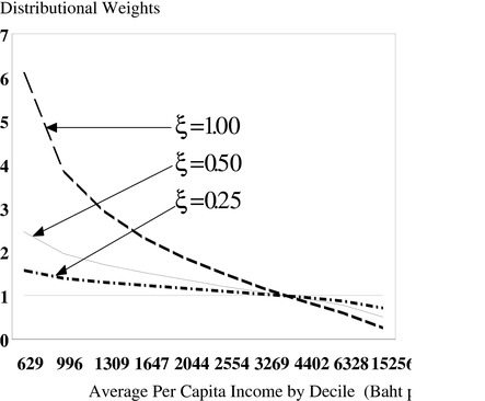
TABLE 6: DISTRIBUTIONAL CHARACTERISTICS FOR THE MAJOR EXPENDITURE CATEGORIES IN THAILAND
|
|
ξ = 0.00
|
ξ = 0.25
|
ξ = 0.50
|
ξ = 1.00
|
|
|
Normalized Distributional Characteristics
|
|||
|
Food
|
1.000
|
1.00
|
1.000
|
1.000
|
|
Alcohol
|
1.000
|
0.882
|
0.835
|
0.762
|
|
Tobacco
|
1.000
|
0.885
|
0.821
|
0.707
|
|
Clothing
|
1.000
|
0.942
|
0.893
|
0.828
|
|
Health
|
1.000
|
0.940
|
0.849
|
0.721
|
|
Electricity and Fuels
|
1.000
|
0.957
|
0.874
|
0.754
|
|
Telecommunications
|
1.000
|
0.888
|
0.799
|
0.660
|
|
Housing and Water
|
1.000
|
0.987
|
0.922
|
0.824
|
|
Entertainment
|
1.000
|
0.904
|
0.801
|
0.659
|
|
Other
|
1.000
|
0.910
|
0.827
|
0.700
|
|
|
|
|||
|
|
SMCFsa
|
|||
|
Alcohol Excise
|
2.311
|
2.038
|
1.930
|
1.761
|
|
Tobacco Excise
|
2.183
|
1.932
|
1.792
|
1.543
|
|
Fuel Excise
|
0.533
|
0.510
|
0.465
|
0.402
|
aBased on the Benchmark parameter values.
The bottom panel of Table 6 shows the SMCFs for the three excise taxes using the distributional characteristics for the three goods. Note that the ranking of the SMCFs is the same as the MCFs—the fuel excise tax always has the lowest social cost, followed by tobacco, and the alcohol excise has the highest SMCF. Consequently, placing higher weights on the losses sustained by lower income groups does not alter the view, based solely on efficiency considerations, that a revenue-neutral increase in fuel excise taxes and a cut in alcohol and tobacco excise taxes would represent an improvement in social welfare.
CONCLUSION
The major contribution of this paper is to expand the Ahmad-Stern framework for evaluating marginal commodity tax reforms by incorporating the most important non-tax distortions that influence the setting of excise taxes on alcohol, tobacco and fuels in Thailand. Some of these distortions, such as environmental externalities and addiction, reduce the social marginal cost of imposing excise taxes; other distortions, such as the exercise of market power by producers of alcohol and tobacco and smuggling, tend to raise the MCFs for these excise taxes. While there is a great deal of uncertainty about the appropriate values for these parameters, our analysis provides a framework within which the net effects of these offsetting distortions can be evaluated. Our results indicate that smuggling, market power, and addiction have potentially large impacts on the MCFs, especially for tobacco taxes, and that interactions with other tax bases is especially important for calculating the MCFs for excise taxes. Our overall conclusion is that the MCFs for alcohol and tobacco excise taxes in Thailand are much higher than for fuel excise taxes and that there would be substantial welfare gain from a revenue-neutral reduction in the excise tax rates on alcohol and tobacco and an increase in fuel excise tax rates.
There are a number of areas where more research and data collection would help in the evaluation of the excise taxes in Thailand. First, the interaction between commodity prices and labour income should be investigated in light of the recent results obtained by West and Williams (2006) for the U.S. Second, the possibility of over-shifting of excise taxes, which has been recorded in the market for alcohol in the U.S. by Young and Bielińska–Kwapisz (2002), should be investigated in Thailand. Third, tourism is an important industry in Thailand, and foreign tourists may bear a significant portion of the excise taxes on alcohol and tobacco. Significant levels of “tax exporting” to tourists might reduce the MCFs for these excise taxes. Finally, businesses and industry pay some of the fuel excise taxes and to the extent that the fuel excises exceed their marginal externality costs, they may create relatively large welfare losses by distorting firm’s production decisions. These effects should also be included in the computation of the MCF for the fuel taxes.
REFERENCES
Ahmad, E. and N. Stern (1984), “The Theory of Reform and Indian Indirect Taxes”, Journal of Public Economics, 25(3): 259-298.
Ahmad, E. and N. Stern (1990), “Tax Reform and Shadow Prices for Pakistan”, Oxford Economic Papers, 42(1): 135-59.
Badenes-Plá, N. and A. Jones (2003), “Addictive Goods and Taxes: A Survey from an Economic Perspective”, Hacienda Pública Española / Revista de Economía Pública, 167(4): 123-153
Bank of Thailand, available at http://www.bot.or.th/bothomepage/databank/EconData/Econ&Finance/.
Bernheim, B. and A. Rangel (2005), “Behavioral Public Economics: Welfare and Policy Analysis with Non-Standard Decision Makers”, NBER Working Paper 11518.
Burgess, R. and N. Stern (1993), “Taxation and Development”, Journal of Economic Literature, 31(2): 762-830
Chaloupka, F., M. Grossman, and H. Saffer (2002), “The Effects of Price on Alcohol Consumption and Alcohol-Related Problems”, Alcohol Research and Health, 26(1): 22-34.
Cnossen, S. (2005), Theory and Practice of Excise Taxation - Smoking, Drinking, Gambling, Polluting, and Driving, Oxford University Press, Oxford.
Cnossen, S. and Smart, M. (2005), “Taxation of Tobacco”, in S. Cnossen (ed.) Theory and Practice of Excise Taxation - Smoking, Drinking, Gambling, Polluting, and Driving, Oxford University Press, Oxford, Chapter 2: 20-55.
Cook, P. and M. Moore (2002), “The Economics of Alcohol Abuse and Alcohol-Control Policies”, Health Affairs, 21(2): 120-133.
Cragg, M. (1991), “Do we care? A Study of Canada’s Indirect Tax System”, Canadian Journal of Economics, 24(1): 124-143.
Dahlby, B. (forthcoming), The Marginal Cost of Public Funds: Theory and Applications, MIT Press, Boston.
Deaton, A. and J. Muellbauer (1980), Economics and Consumer Behavior, Cambridge University Press, New York.
Decker, S. and A. Schwartz (2000), “Cigarettes and Alcohol: Substitutes or Complement?”, NBER Working Paper No. 7535.
Decoster, A. and E. Schokkaert (1990) “Tax Reform Results with Different Demand Systems” Journal of Public Economics 41(3): 277-296.
Delipalla, S. and O. O’Donnell. (2001), “Estimating Tax Incidence, Market Power and Market Conduct: The European Cigarette Industry”, International Journal of Industrial Organization 19(6): 885-908.
The Economist (2006), “The Avuncular State”, Special Report on the New Paternalism, April 26th: 67-69.
Feldstein, M. (1972), “Distributional Equity and the Optimal Structure of Public Prices”, American Economics Review, 62(1): 32-36.
Galbraith, J.W. and M. Kaiserman (1997), “Taxation, Smuggling and Demand for Cigarettes in Canada: Evidence for Time-Series Data”, Journal of Health Economics, 16(3): 287-301.
Goel, R. and M. Morey (1995), "The Interdependence of Cigarette and Liquor Demand", Southern Economic Journal, 62(2): 451-459.
Grossman, M. (2004), “Individual Behaviors and Substance Use: The Role of Price”, NBER working paper 10948, December.
Grossman, M., J. Sindelar, J. Mullahy, and R. Anderson (1993), “Policy Watch: Alcohol and Cigarette Taxes”, Journal of Economic Perspectives, 7(4): 211-222.
Gruber, J and B. Kőszegi (2004), “Tax Incidence When Individuals Are Time-Inconsistent: The Case of Cigarette Excise Taxes”, Journal of Public Economics, 88(9-10): 1959-1987.
Gruber, J, A. Sen, and M. Stabile (2002), “Estimating Price Elasticities when there is Smuggling: The Sensitivity of Smoking to Price in Canada”, NBER working paper 8962.
Gruber, J. and S. Mullainathan (2005), “Do Cigarette Taxes Make Smokers Happier”, Advances in Economic Analysis and Policy, 5(1): Article 4.
Guindon, G., S. Tobin, and D. Yach (2002), “Trends and Affordability of Cigarette Prices: Ample Room for Tax Increases and Related Health Gains”, Tobacco Control, 11: 35-43.
International Telecommunication Union (2002) “Bits and Bahts: Thailand Internet Case Study,” Geneva, Switzerland, March. available at www.itu.int/asean2001/reports/material/THA%20CS.pdf
Irvine, I. and W. Sims (1993), “The Welfare Effects of Alcohol Taxation” Journal of Public Economics, 52(1): 83-100.
Jones, A. (1989), "A Systems Approach to the Demand for Alcohol and Tobacco", Bulletin of Economic Research, 41(2): 85-105.
Joossens, L., F. Chaloupka, D. Merriman, and A. Yurekli, (2000), “Issues in the Smuggling of Tobacco Products”, in P. Jha and F. Chaloupka (eds.) Tobacco Control in Developing Countries, Oxford University Press, Oxford, Chapter 16, 393-406.
Kenkel, D. (1996), “New Estimates of the Optimal Tax on Alcohol”, Economic Inquiry, 34(2): 296-319.
Leung, S. and C. Phelps (1993), “My Kingdom for a Drink...? A Review of Estimates of the Price Sensitivity of Demand for Alcoholic Beverage”, in M.E. Hilton and G. Bloss (eds.), Economics and the Prevention of Alcohol Related Problems, Proceedings of Workshop on Economics and Socioeconomic Issues in the Prevention of Alcohol-Related Problems. October 10-11, 1991.
Liberati, P. (2001), “The Distributional Effects of Indirect Tax Changes in Italy”, International Tax and Public Finance, 8(1): 27-51.
Madden, D. (1995), “Labour Supply, Commodity Demand and Marginal Tax Reform”, Economic Journal, 105(429): 485-497.
Manning, W., E. Keeler, J. Newhouse, E. Sloss, and J. Wasserman (1989), “The Taxes of Sin: Do Smokers and Drinkers Pay Their Way?”, Journal of American Medical Association, 261: 1604-1609.
Merriman, D., A. Yurekli, and F. Chaloupka (2000), “How Big is the Worldwide Cigarette Smuggling Problem?”, in P. Jha and F. Chaloupka (eds.), Tobacco Control in Developing Countries, Oxford University Press, Oxford, Chapter 15: 365-392.
Ministry of Public Health, (2004), Public Health in Thailand 1999-2004. Ministry of Public Health, Bangkok.
National Statistical Office, (2002), Socio-Economic Survey Data Tape 2002, Bangkok.
National Statistical Office, (2003), Health and Welfare Survey Data Tape 2003, Bangkok.
Newbery, M. (2005), “Road User and Congestion Charges” in S. Cnossen (ed.) Theory and Practice of Excise Taxation - Smoking, Drinking, Gambling, Polluting, and Driving, Oxford University Press, Oxford, Chapter 7: 193-229.
Norton, D. (1988), “On the Economic Theory of Smuggling”, Economica 55(217): 107-118.
O’Donoghue, T. and M. Rabin, (2006), “Optimal Sin Taxes”, Journal of Public Economics, 90(10-11):1825-1849.
Parry, I. (2003), “On the Costs of Excise Taxes and Income Taxes in the UK”, International Tax and Public Finance, 10(3): 281-304.
Parry, I. and K. Small (2005), “Does Britain or the United States Have the Right Gasoline Tax?”, American Economic Review, 95(4): 1276-1289.
Pattamasiriwat, D. (1989), “A Study of Consumption Pattern using National Income Account”, Chulalongkorn Journal of Economics, 1(2): 244-264. (in Thai).
Poapongsakorn, N., K. Charnvitayapong, D. Laovakul, S. Suksiriserekul and B. Dahlby (2000), “A Cost-Benefit Analysis of the Thailand Taxpayer Survey”, International Tax and Public Finance, 7(1): 63-82.
Pogue, T. and L. Sgontz (1989), “Taxing to Control Social Costs: The Case of Alcohol”, American Economic Review, 79(1): 235-243.
Ray, R. (1997), “Issues in the Design and Reform of Commodity Taxes: Analytical Results and Empirical Evidence”, Journal of Economic Surveys, 11(4): 353-388.
Rosenberger, R. and J. Loomis (2003), “Benefit Transfer”, in P. Shamp, K. Boyle and T. Brown (eds.), A Primer on Nonmarket Valuation. Kluwer Academic Publishers, Dordrecht, Chapter 12, 445-482.
Santoro, A. (no date), “Marginal Commodity Tax Reforms: A Survey” working paper, University of Milan-Bicocca.
Sarntisart, I. (2003), Economic Analysis for Tobacco Control in Thailand. A Report for Discussion “Health, Nutrition and Population, Tobacco Free Initiative,” World Health Organization. (in Thai)
Smith, S. (2005), “Economic Issues in Alcohol Taxation” in S. Cnossen (ed.), Theory and Practice of Excise Taxation - Smoking, Drinking, Gambling, Polluting, and Driving, Oxford University Press, Oxford, Chapter 3, 56-83.
Sriyookrat, P. (2001), A Study of Market Structure and Factor Affecting Demand for Alcoholic Beverages in Thailand. A Thesis for Master of Science (Agricultural Economics), Department of Agricultural and Resource Economics, Kasetsart University.
Sunley, E., A. Yurekli, and F. Chaloupka (2000), “The Design, Administration, and Potential of Tobacco Excises” in P. Jha and F. Chaloupka (eds.), Tobacco Control in Developing Countries, Oxford University Press, Oxford, Chapter 17, 409-426.
Tanzi, V., and H. Zee (2000), “Tax Policy for Emerging Markets: Developing Countries”, National Tax Journal, 53(2): 299-322.
TDRI (2005), Alcoholic Beverage Consumption in Thailand. Thailand Development Research Institute, Bangkok (in Thai).
TDRI (2006), “An Impact Assessment of Alcoholic Beverage Tax on Its Price and Consumption”, Thailand Development Research Institute, Bangkok, (in Thai).
Thai Beverage PCL. (2005), Prospectus: ThaiBev PCL. available at www.bangkokbiznew.com/2005/ special/beerchang/ downloaded on Feb. 21, 2006 (in Thai).
Usher, D. (1986), “Tax Evasion and the Marginal Cost of Public Funds”, Economic Inquiry, 24(4): 563-586.
Wade, S. (2003), “Price Responsiveness in the AEO2003 NEMS Residential and Commercial Buildings Sector Models”, Energy Information Administration Publication. (www.eia.doe.gov/oiaf/analysispaper/elasticity/pdf/buildings.pdf downloaded on Aug. 30, 2006).
West, S. and R. Williams III (2007), “Optimal Taxation and Cross-Price Effects on Labor Supply: Estimates of the Optimal Gas Tax”, Journal of Public Economics, 91(3-4): 593-617.
Young, D. and A. Bielińska–Kwapisz (2002), “Alcohol and Beverage Prices” National Tax Journal, 55(1): 57-73.
[†]The authors would like to thank Patanayut Santiyanont and Suwimon Fakthong for their efficient research assistance and especially to David Ryan for his advice on econometric issues. We are grateful to an anonymous referee for his/her comments. We are responsible for any errors or omissions. Major funding for this research project came from the Canadian International Development Agency (CIDA). Other funding was provided by the Human Resources and Social Development Program, Thailand Development Research Institute.
[∗] Senior Research Specialist at the Thailand Development Research Institute, Bangkok, Thailand. Email: worawan@tdri.or.th.
∗∗Professor at the Department of Economics and Fellow of the Institute of Public Economics, University of Alberta, Alberta, Canada. Email: bdahlby@ualberta.ca.
[1] Calculations based on data in Tanzi and Zee (2000, Table 2, p.304). See also Burgess and Stern (1993, Table 5, p.773) on developing countries’ reliance on goods and services taxation.
[2] This section is based on Dahlby (forthcoming, Chapters 2 and 3).
[3] It further assumed that the taxes do not affect relative input prices. This is an admittedly strong assumption given that some fuel excise taxes are paid by businesses.
[4] Bernheim and Rangel (2005, p.39).
[5] In general, it is important to distinguish between ad valorem taxes and per unit taxes in evaluating the MCF from taxing a monopolist’s product because as is well known a monopolist’s price response differs for these two types of taxes. See Dahlby (forthcoming, Chapter 3). For our purposes, because the Thai Tobacco Company is a state-owned monopoly, this distinction can be ignored as will be shown below.
[6] For a recent application of this methodology to commodity tax reform in Italy, see Liberati (2001).
[7] A recent study by Decker and Schwartz (2000) using household level data from the U.S. indicated that the demand for cigarettes declines when alcohol prices increase while the demand for alcohol increases when the price of cigarettes increase. An early study using aggregate US data by Goel and Morey (1995) had indicated that alcohol and tobacco were substitutes, while a study using UK data by Jones (1989) indicated that tobacco was a complement for alcohol. Gruber, Sen and Stabile (2002) based on Canadian data found that higher cigarette prices reduced alcohol consumption.
[8] See N. Badenes-Plá and Jones (2003, Table 2, p.139) for a summary of empirical estimates of the elasticity of cigarette consumption which are in the -0.40 to -0.60 range.
[9] See Parry and Smart (2005, p. 1283).
[10] Madden calculated the marginal revenue cost of increasing welfare, which is the inverse of the MCF.
[11] See Dahlby (forthcoming, Chapter 3).
[12] Parry (2003) has provided an extensive review of the empirical literature on the externalities generated by the consumption of gasoline, alcohol, and cigarettes in the United States and the United Kingdom. While there is still a great deal of uncertainty concerning the magnitudes of these parameters, Parry’s choices for his base case estimates seem reasonable, but their applicability to Thailand is unknown. Based on his review of the literature, Parry concluded that tobacco products impose the largest harmful externalities, representing 28.3 percent of the consumer price of the product, followed by petrol at 17.8 percent, and alcohol at 11 percent of the product price. It should be noted that Parry treated all externalities as direct consumption externalities even though his discussion and the literature indicate that these externalities, especially for smoking and alcohol consumption, take the form of higher public expenditures on health care, and in our framework would be included in the δG parameters.
[13] For further discussion of the externalities caused by alcohol consumption and tax policies to deal with these issues, see Pogue and Sgontz (1989), Grossman et al. (1993), Irvine and Sims (1993), Kenkel (1996), Cook and Moore (2002), and Chaloupka, Grossman, and Saffer (2002) and Grossman (2004).
[14] This benefit transfer technique (the value transfer method) is used to convert the study site values (U.K in this case) to policy site values (Thailand in this case). The conversion using real per capita GDP is widely applied in environmental assessment in Thailand. See Rosenberger and Loomis (2003) for more details of the technique.
[15] These figures are from the Health and Welfare Survey (HWS) in 2003. The survey is conducted by National Statistical Office of Thailand. It interviews health status, healthcare insurance coverage, healthcare expenditure, and health related behaviour.
[16] From Health and Welfare Survey in 2003.
[17] See Delipalla and O’Donnell (2001) on the concentration of EU cigarette markets.
[18] (For a summary of market competition, see in an appendix available from the authors upon request.)
[19] In the TDRI study the price elasticities for color liquor, white liquor, imported liquor, beer and wine were -1.56, -2.73, -0.61, -2.68 and -0.60 respectively.
[20] Delipalla and O’Donnell (2001) used a conjectural variations framework to estimate the responsiveness of cigarette prices to tax changes in European countries. Their estimates of the tax shifting parameters were consistent with the theoretical prediction that ad valorem taxes produce smaller price increases than per unit taxes in an imperfectly competitive market. The ratio of the tax shifting effects for per unit and ad valorem taxes yields an estimate of the market power distortion of 0.219 if the price elasticity of demand for cigarettes is -0.40.
[21] If one assumes that the mobile phone market is a Cournot duopoly, then the δM parameter could be calculated as 0.5 (1/0.183)0.35 = 0.956 where the 0.5 is one divided by the number of firms and 0.183 is our estimate of the elasticity of demand for telecom services and 35 percent is the mobile phone share of the total market for telecom services (International Telecommunication Union (2002), Table 2.3). This estimate of the market power distortion is very high because our estimate of the demand elasticity for telecommunications is so low. We believe the range of values that we have used in the calculation is more realistic.
[22] See Smith (2005, p.77) for the UK figure.
[23] In July 2002, one Baht was worth approximately 0.024 US dollars.
AustLII:
Copyright Policy
|
Disclaimers
|
Privacy Policy
|
Feedback
URL: http://www.austlii.edu.au/au/journals/eJlTaxR/2007/6.html